Tech Article | 23/08

Ansys – on the path to artificial intelligence?

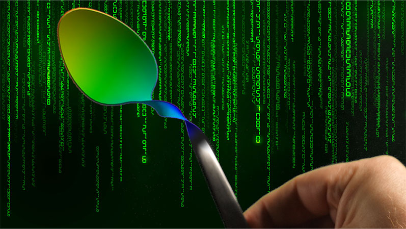
In “The Matrix”, Neo lives in a virtual world where spoons can bend, and physical boundaries can be exceeded. Ok - we aren’t quite there yet, but the rapid progress of physics-based simulation predicts that we will be able to do incredible things in the near future. Let’s now immerse ourselves in an “entryway” in which a trained system “bends your spoon” in real time.

Workflows in Ansys – similarities to artificial intelligence

Let’s start with a classification. Similar to an AI like ChatGPT, the quality of the prediction of a simulation model depends largely on having a good database, which then needs to be trained. As engineers, however, we don't have big data with billions of parameters. In the worst case, we only have a few hundred variants of a design as well as their simulation results describing the physical behavior that form the database. But this is quite manageable in comparison. In our case, we’re able to bend and twist our spoon in all possible directions using the parameters we have. It’s very simple: just a click on the parameter box and the values can be changed using the parameter set (see picture below).

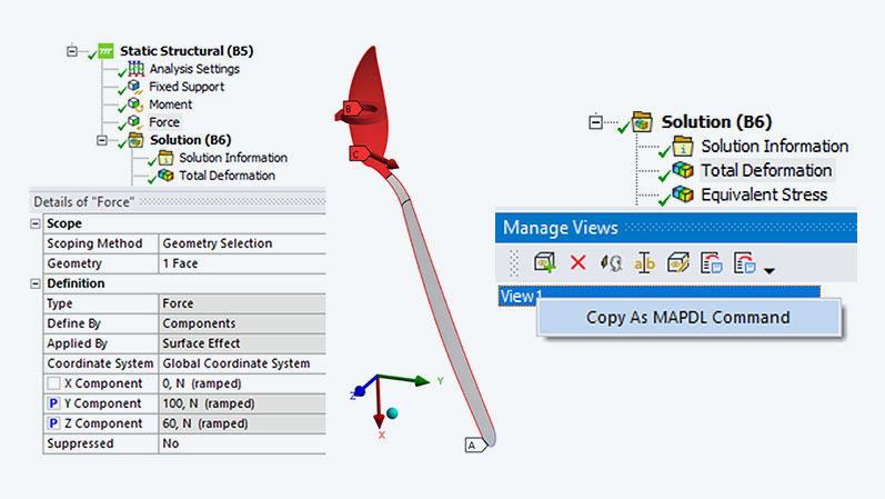
The database is created when we generate and calculate variants using these parameters. Initially, it’s difficult to interpret the resulting maximum deformation values. However, images can help. Did you know that you can save an additional image for each variant? This can be done with APDL, for example:

! COPY VIEW INFORMATION HERE
/SHOW,PNG $ PLNSOL,U,SUM $ /SHOW,CLOSE

The information for the desired view can be obtained via the View Manager (see picture below). By right clicking, you can generate a view and copy the APDL code. With the optiSLang Data Send node, you can specify that these images should not be deleted.

Or you can use an “After Post” Python code snippet:

import os
solveDir = solution.WorkingDir
camera = Graphics.Camera
camera.SetSpecificViewOrientation(ViewOrientationType.Bottom)
camera.SetFit()
viewOptsRes = Graphics.ViewOptions.ResultPreference
viewOptsRes.ContourView = MechanicalEnums.Graphics.ContourView.ContourBands
viewOptsRes.ExtraModelDisplay = MechanicalEnums.Graphics.ExtraModelDisplay.UndeformedWireframe
for myResult in solution.GetChildren(DataModelObjectCategory.Result, False):
fpath = os.path.join(solveDir,myResult.Name + ".jpg")
myResult.Activate() Graphics.ExportImage(fpath,
GraphicsImageExportFormat.JPG)

Parameterization in Ansys Mechanical | © CADFEM Germany + How to get the APDL code with the View Manager | © CADFEM Germany

What is important for a trained data model (DL) ?

Next, we can use this data – let’s call it the deep learning phase – to train a metamodel that ultimately predicts all conceivable maximum deformations. Is the deformation of the spoon tip greater when equal force is applied to the side as opposed to the back? How far will it bend if it is twisted with a moment at the same time? Thanks to our metamodel, we are now able to provide this answer live and without further simulation. Three points are important here:

Data security: We want to protect the generated data. Nothing should be sent and processed over the Internet. Instead, everything should be kept in our computing environment. No one else should know your spoon secret.
Prediction quality: How good is my trained model? Does it just deliver a good-looking result? To evaluate the quality, we can use the so-called coefficient of prognosis, which tells us whether the model can be used or whether it should be trained further.
Traceability: What logic does AI use to arrive at its answer? This is also an issue we need to consider here. The metamodel explains the relationships between the parameters, which contributes to understanding when interpreting the results. In other words: transparency – not a black box.

Schematic setup for the generation and evaluation of a trained metamodel | © CADFEM Germany; Representation of the maximum displacement as a function of applied load and moment | © CADFEM Germany; Deformation of the twisted and bent spoon | © CADFEM Germany

Can metamodels also be generated for curves?

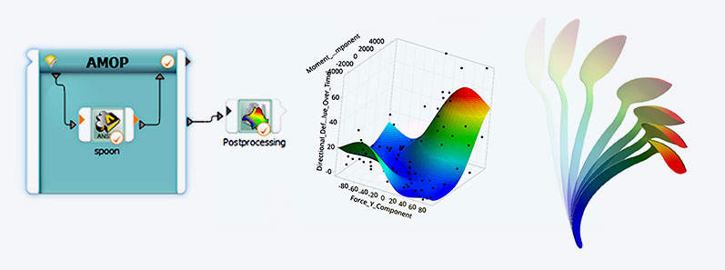
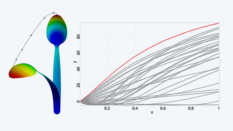
When you look at the spoon, the next thing you might want to see is the path taken by the tip of the spoon. So, let’s move on to the next dimension, away from the less exciting scalar variables to the more interesting signals. For this, the result file of each variant is read in and the curve of the displacement components of the node at the spoon tip is saved in so-called “channels”. Signals can be generated from these and a signal metamodel can be trained. Now it’s possible to identify the path that the tip would take in any situation.

But that’s not all – we can also identify the parameters that determine this path. If we know which parameters are responsible for the curve characteristics or for the respective section of the curve, we can use this information to continue working only with these parameters. We ignore the unimportant parameters, so to speak, thus saving time and can even achieve higher coefficients of prognosis using this “pre-filter”.

Deformation path of the bent spoon | © CADFEM signal plot: various deformation paths of the spoon tip mapped in the x-y plane © | © CADFEM Germany

Transparency in data analysis builds trust | © Adobe Stock

How can a metamodel for a field be trained?

But is that all? No. Not only do we want to observe the tip of the spoon, we also want to be able to describe the displacement of every single point on the spoon. So, off we go into the next dimension - the world of so-called random fields! For this, we don't train a metamodel or signal metamodel for individual nodes, but rather a field metamodel for our entire structure.

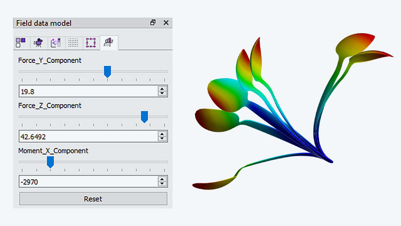
This is then able to describe the complete deformation behavior of the spoon under all possible force and moment scenarios – in real time, again without simulation.

Since this is obviously also an approximation model, questions about the quality of the deformation fields inevitably arise again. This can be displayed directly on the structure in the form of a color plot so that you don't have to blindly trust the results. Because it's like with AI - if you blindly trust it, you've already lost. It's important to always question things. In this case, we do this by comparing the standard deviations of the imported random fields with the generated random field model.

What can a field metamodel be used for?

Now that we have a proven high-quality field metamodel, we’re able to use it. So, ask questions and consider the answers. To make this quick and easy, there are so-called “field inspectors”, which are sliders for the input parameters. These can be used to set the desired values (which are the questions) in a flash. The answers come live in the form of simulation images.

What we have done for the spoon can be applied to all fields that can be calculated in Ansys

stress fields
temperature fields
electromagnetic fields
flow fields and much more.

The benefit is clear: once trained, you can ask questions and get answers immediately. Similar to ChatGPT, this saves an enormous amount of time.

Field inspectors to quickly “ask the question” | © CADFEM Germany; Various answers to the questions asked | © CADFEM Germany

optiSLang for the use of DL or ML in Ansys

But wait... what if the database expands? In other words, if there are new findings that would make my model even smarter? That’s where the Reevaluate Workflow and the technology of the so-called Adaptive Metamodel of Optimal Prognosis (AMOP) come into play. These allow you to subsequently extract additional, initially seemingly unimportant result variables from your data sets and also train the metamodel further. This predictive analytics approach allows your thoughts to wander even further – towards integrated live feedback on websites, system simulations, or digital twins. So, all possibilities are on the table.

Now is the time to make a decision: you can carry on as before, or we can show you how deep the rabbit hole goes. Get started with a free introduction to this topic and then follow the path that leads to the CADFEM Learning Subscription. In the eLearning for “optiSLang”, you will acquire essential knowledge and can build on it with the CADFEM Let’s Simulate series on “Linking Processes” and “Statistics on Structures”. This is exactly what you need to implement your own processes! So, don’t rely on the tricks of well-known “spoon bending mentalists”, instead become one with the spoon yourself!